Florida Poly Thesis Template
Author:
Chris Kelley
Last Updated:
3년 전
License:
Creative Commons CC BY 4.0
Abstract:
Template for Florida Poly thesis formatting.

\begin
Discover why over 25 million people worldwide trust Overleaf with their work.

\begin
Discover why over 25 million people worldwide trust Overleaf with their work.
%%
%% THESIS/DISSERTATION TEMPLATE FOR FLORIDA POLYTECHNIC UNIVERSITY
%%
%% This example is written by Chris Kelley, edited from a template for the University of Alabama.
%%

%% Use the fputhesis document class
\documentclass[thesis]{fputhesis}

%% Basic packages you'll probably want to use.
\usepackage{graphicx}                 %% For using \includegraphics{}
\usepackage{cite}                     %% For sorting/collapsing citations.
%\usepackage{subfigure}
\usepackage{float}
\usepackage{amsmath}
\usepackage{multirow}
\usepackage{color}                    %% For colors used in listings.
\usepackage{listings}                 %% Code listings (for engineers)
\usepackage[numbers]{natbib}

\newcommand{\Vol}{\rotatebox[origin=c]{180}{\ensuremath{A}}}

%% Includes
%\input{inc/glossary.tex}
% TODO: If you have any special commands defined, include them here.
\usepackage[titletoc]{appendix}%


%% Required parameters (these default to undefined)
\author{Student Name}       %% Your name!
\university{Florida Polytechnic University}
\gradyear{Spring \the\year}
\place{Lakeland, Florida}
\degree{Master of Science in Engineering}   %% Change to suit your degree.
\prevdegree{Bachelor of Science, Mechanical Engineering}   %% Change to suit your previous degree.
\department{INSERT YOUR DEPARTMENT NAME HERE}   %% Change to suit your department.


%% The people on your committee.
\adviser{Dr. T. Adviser}   %% Your adviser/committee chair!\
\memberA{Dr. A. Member}
\memberB{Dr. B. Member}
\provost{Dr. T. Provost}


%% Note the use of \and to create line breaks and the
%% inverted pyramid style requested by the graduate school.
%% You have to do this manually. Sorry.
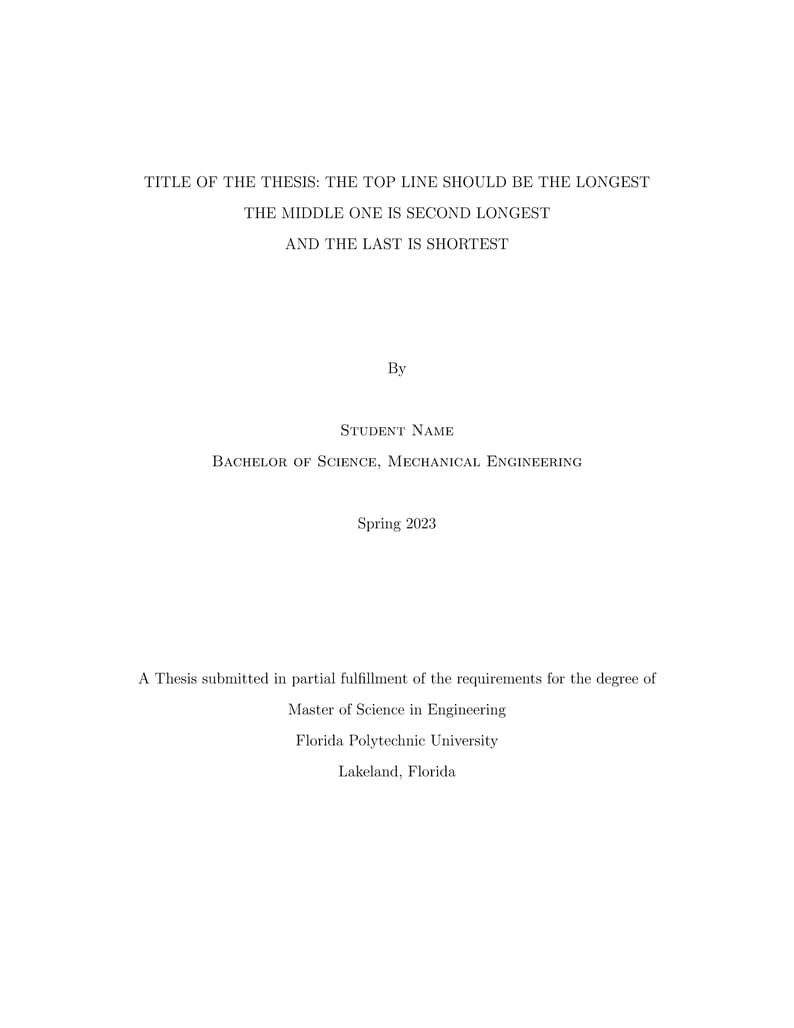
\title{Title of the thesis: the top line should be the longest \and
  the middle one is second longest \and
  and the last is shortest}


%% These are body text paragraphs to be placed in the front matter.
\abstract{
Type your abstract here.

}

\dedication{
Type or input{} your dedication here.
}

\acknowledgments{
Type your acknowledgments here.
}


\begin{document}

%% Makes the title, abstract, dedication, table of contents, etc.
%% Must be before \begin{body}
\makefrontmatter

%% BODY PORTION
%% The bulk of your thesis.
%% Begin your \chapter's here.

\begin{body}


%% Body chapters.
\chapter{INTRODUCTION}
This template follows the thesis format guidelines from the Florida Poly Thesis and Project Manual. This template also includes sample figures, equations, etc. to demonstrate how key elements are included in Latex. For example, check the code for Fig.~\ref{trapplate} to see how to insert a figure. Also, check this sentence for how to insert in-text citations~\cite{Kelley2017JIMSS}. You define the callout name and reference details in the ``.bib'' file. You can also insert multiple citations at the same instance~\cite{Kelley2017JIMSS,Kelley2019Scitech,Preumont2006M,IEEEstandard,Kauffman2012PhD}. Leave one or more blank lines between blocks of text to start a new paragraph (you can have as many blank lines as you want---they do not affect document format).

Each chapter also includes the description for what to include for that chapter as provided by the Thesis and Project Manual. The chapter titles are those listed by the Thesis and Project Manual, but different chapter titles often make more sense for many STEM theses. A general framework typically includes an introduction for Chapter 1, background/literature review for Chapter 2, and conclusions for the final chapter. In between, there are 2--4 chapters that cover the approach, methods, results, and discussion---sometimes these chapters have topic-specific titles (e.g., ``Computational Model'').


\section{Poly Manual Description}
The introduction chapter should emphasize the purpose of the study and summarize the background and importance of this research. This chapter should also clearly state the hypothesis and the objectives of the research. Finally, this chapter should introduce the user to the outline of the thesis.


\begin{figure}[t]
\centering
\includegraphics[scale=0.4]{dimensionedplate3}
\caption{Representative turbomachinery blade}\label{trapplate}
\end{figure}


\chapter{LITERATURE SURVEY}
Type your chapter here...


\section{Here is a Section Title}
Here is some text. Let's use a subsection for the Thesis and Project Manual chapter description this time.


\subsection{Poly Manual Description}
The literature review will summarize the existing research in the field with references to these research studies and their authors. At the end of the literature review, clearly state the identified gaps in the existing research solutions and address these gaps by this thesis. In other words, you are introducing the reader to your work in the next chapter.


\chapter{RESEARCH METHODOLOGY}
Take a look at Table~\ref{proptable}. It shows how you can make a table in Latex. You can also make your table elsewhere and insert the image in a similar way as inserting an image for a figure. Note that you upload all your images using the ``Upload'' tool on the top left corner of Overleaf (it has an arrow pointing up).


\begin{table*}[t]
 \centering
\caption{Parameters used in experimental setup.}\label{proptable}
\begin{tabular}{ |c|c|c|c|c|c|c|c|c| }
\hline
%\multicolumn{8}{|c|}{Cantilever Beam Properties}\\ \hline
		  &$a$ (mm)          &$h$ (mm) &$E$ (GPa)     &$\nu$   &$\rho$ ($\text{kg/m}^2$)  &$\varepsilon_\text{rel}$   	   \\ \hline
\textbf{Plate}		    &128     &2.03  &68.9  &0.31  &2750  &-            \\ \hline
\textbf{Piezo}		&34.3     &0.267  &59.8  &0.31  &7500  &1953                \\ \hline
\end{tabular}
\end{table*}


\section{Poly Manual Description}
This chapter will provide details on the chosen methods, designs, measures, and philosophy behind these choices. In addition, this chapter should include a description of any conduct experiment.


\chapter{RESULTS}
Type your chapter here. Let us show some examples of inserting equations here. Sometimes we want to write equations or math symbols in the text, like this: $c^2=\sqrt{a^2+b^2}$. However, most of the time we want to insert numbered equations, like this:
\begin{equation}\label{coupling}
k^2=\frac{\text{electrical energy}}{\text{imposed work}}=\frac{\omega^2_{\text{oc}}-\omega^2_{\text{sc}}}{\omega^2_{\text{oc}}}
\end{equation}
Do not include a blank like after the equation if you want to continue in the same paragraph. You can easily refer back to an equation: go check out Eqn.~\eqref{coupling}. Now I will paste in some text and equations from a previous paper that demonstrate a variety of math symbols, structures, etc.


\section{Sample equations}
Analysis of the strain energy produces the bending stiffness matrix, which is split into the contribution from the plate $[K_o]$ and the contribution from the piezoelectric patches $[K_p]$. The stiffness from the plate is:
\begin{equation}\label{Stiffness}
[K_o]_{rsuv}=\frac{Eh^3}{12(1-\nu^2)}(I_1+I_2+I_3+I_4+I_5) \\
\end{equation}
where Appendix A includes the integrals $I_1$ through $I_5$, which have the form:
\begin{equation}
I_i=C_i\int_0^a x^{n_1}(b_1+\frac{b_2-b_1}{a}x)^{n_2} \text{d}x
\end{equation}
The integration over $x$ may be carried out analytically in MATLAB using polynomial functions. Now, integrating over the piezoelectric material volume produces:
\begin{align}\label{PiezoStiffness}
\begin{split}
[K_p]&_{rsuv}=\sum_{p=1}^P \frac{E_p}{12(1-\nu_p)^2} (3h^2 h_p+6h h_p^2+4h_p^3) \\
&\times (I_{1p}+I_{2p}+I_{3p}+I_{4p}+I_{5p})
\end{split}
\end{align}

The total bending stiffness matrix from the strain energy is the summation of the plate and piezoelectric patch matrices:
\begin{equation}
[K]=[K_o]+[K_p]
\end{equation}
In addition to these terms, the stiffness matrix must also incorporate the stiffening associated with in-planes loads induced by centrifugal loading.


\subsection{Electrical and Coupling Stiffness Matrices}
Analysis of electrical energy and coupled energy leads to electrical and coupled stiffness matrices. The electrical stiffness matrix is diagonal; the $P$ entries are the equivalent capacitances of the piezoelectric patches:
\begin{equation}\label{ElectricalStiffness}
[K_e]_{pp}=\frac{\varepsilon_p A_p}{h_p}
\end{equation}
The coupled energy produces the coupling stiffness matrix:
\begin{equation}\label{CoupledStiffness}
\begin{split}
[K_c]_{prs}=\sum_{p=1}^P e_{31p} \frac{h+h_p}{2} \left(\frac{r+1}{s} \frac{(x_{2p}^r-x_{1p}^r)(y_{2p}^s-y_{1p}^s)}{a^{r+1}b_2^{s-1}}\right. \\
\left. +\frac{s-1}{r+2} \frac{(x_{2p}^{r+2}-x_{1p}^{r+2})(y_{2p}^{s-2}-y_{1p}^{s-2})}{a^{r+1}b_2^{s-1}}\right)
\end{split}
\end{equation}
Note the second term in $[K_c]_{prs}$ is equal to zero when $s \leq 2$.


\subsection{Mass Matrix}
Analysis of the kinetic energy produces the mass matrix. Similar to the bending stiffness, the mass matrix includes plate and piezoelectric patch components. The plate contribution to the mass matrix is:
\begin{align}\label{Mass}
&[M_o]_{rsuv} = \frac{2\rho h}{(s+v-1)a^{r+u+2}b_2^{s+v-2}}I_M \\
&I_M =
\begin{cases}
\int_0^a x^{r+u+2}(b_1+\frac{b_2-b_1}{a}x)^{s+v-1} \text{d}x & \text{for } s+v \text{ even} \\
0 & \text{for } s+v \text{ odd}
\end{cases}
\end{align}
The piezoelectric contribution to the mass matrix is:
\begin{align}
[M_p]_{rsuv}&=\sum_{p=1}^P C_{Mp} (x_{2p}^{r+u+3}-x_{1p}^{r+u+3})(y_{2p}^{s+v-1}-y_{1p}^{s+v-1}) \\
C_{Mp}&=\frac{\rho_p h_p}{(r+u+3)(s+v-1)a^{r+u+2}b_2^{s+v-2}}
\end{align}
Summation of these components produces the mass matrix:
\begin{equation}
[M]=[M_o]+[M_p]
\end{equation}


\subsection{Equations of Motion}
The energy formulations enable calculation of the equations of motion via Lagrange's equation:
\begin{equation}
\frac{\text{d}}{\text{d}t}\left(\frac{\partial T}{\partial \{\dot{q}\}}\right)+\frac{\partial(U_{\text{strain}}+U_{\text{elec}}+U_{\text{coupled}})}{\partial \{q\}}=\frac{\partial \delta W}{\partial \{ \delta q \}}
\end{equation}
Here, $\delta W$ is the virtual work performed by generalized mechanical and electrical external forces ($F_m$ and $F_e$, respectively). Inserting energy terms, solving, and adding a damping matrix $[C]$ results in the equations of motion:
\begin{equation}
\begin{bmatrix} M & 0 \\ 0 & 0 \end{bmatrix}
\begin{Bmatrix} \ddot{q}_m \\ \ddot{q}_e \end{Bmatrix}
+\begin{bmatrix} C & 0 \\ 0 & 0 \end{bmatrix}
\begin{Bmatrix} \dot{q}_m \\ \dot{q}_e \end{Bmatrix}
+\begin{bmatrix} K & -K_c^t \\ K_c & K_e \end{bmatrix}
\begin{Bmatrix} {q}_m \\ {q}_e \end{Bmatrix}
=\begin{Bmatrix} F_m \\ F_e \end{Bmatrix}
\end{equation}
where inserting electrical boundary conditions produces a non-singular mass matrix.


\section{Poly Manual Description}
This chapter contains the result of the thesis. If possible, organize the thesis’s results into figures. Otherwise, organize the results into tables. Finally, divide the results into sections and subsections based on the research questions they address.


\chapter{DISCUSSIONS}
Type your chapter here. See the (commented out) code below to check out how to insert a figure with subfigures (subfigure package also commented out in preamble). The code throws an error, but still works... I think the ``subfigure'' package may be obsolete now and there is another way to insert subfigures. In any case, this code does work if you need it.

%\begin{figure*}[t]
%\centering
%\subfigure[Campbell diagram]{\includegraphics[scale=1]{figure1}}\hfill
%\subfigure[RFD switching concept]{\includegraphics[scale=1]{figure2a}}\hfill
%\subfigure[RFD vibration reduction]{\includegraphics[scale=1]{figure2b}}
%\caption{Resonance frequency detuning switches stiffness states to essentially detune the natural frequency from the excitation frequency}\label{RFDfig}
%\end{figure*}


\section{Poly Manual Description}
This chapter contains the analysis, explanations, and discussions of the results. It should also include statements whether the results support the hypothesis or not, with some reasoning if it does not.


\chapter{CONCLUSION}
Type your chapter here...


\section{Poly Manual Description}
This chapter should be a summary of the study indicating whether the study met its goals or not.


\chapter{FUTURE WORK}
Type your chapter here...


\section{Poly Manual Description}
This chapter is a recommended optional chapter. It will present the possible future research paths that will build on this study.


%% Currently adding the references to the table of contents is not automatic
%% So we are forced to do it manually.

%% TODO: This is not a fix. This line has to come after the \chapter command
%% in order for the correct page to be inferred for the table of contents.
\renewcommand{\bibsection}{\topskip=1in\chapter*{REFERENCES}\topskip=0in \addcontentsline{toc}{chapter}{REFERENCES}}

%% Generates the bibliography.
\singlespacing
\bibliographystyle{IEEEtranbib}
\bibliography{thesis-template}


\doublespacing
\begin{appendices}
\addtocontents{toc}{\setlength{\cftchapnumwidth}{1em}}
\renewcommand{\appendixname}{APPENDIX}
\addtocontents{toc}{\setcounter{tocdepth}{0}}
\addtocontents{toc}{\protect\renewcommand{\protect\cftchappresnum}{}}

\chapter{INSERT TITLE}
See below for more pasted code with various equations.

\section{More Sample Equations}
The assumed modes method approximates the transverse displacement $w$ as a summation of assumed shapes weighted by generalized coordinates $q_{rs}$:
\begin{equation}
w(x,y,t)=\sum_{r=1}^R \sum_{s=1}^S q_{rs}(t) \varphi_{X,r}(x) \varphi_{Y,s}(y)
\end{equation}
For this study, the assumed shapes in the $x$- and $y$- directions are:
\begin{align}
\varphi_{X,r}(x) &=\left(\frac{x}{a}\right)^{r+1} \\
\varphi_{Y,s}(x) &=\left(\frac{y}{b_2}\right)^{s-1}
\end{align}
The model includes $R$ shapes in the $x$-direction and $S$ shapes in the $y$-direction. These assumed shapes in each direction form $M$ combined assumed shapes for the entire plate:
\begin{align}
\varphi_m(x,y)&=\varphi_{X,r}(x) \varphi_{Y,s}(y) \\
m&=(r-1)S+s \label{meq} \\
w(x,y,t)&=\sum_{m=1}^M q_{m}(t) \varphi_{m}(x,y)
\end{align}


Although other assumed shapes might provide better convergence, these shapes offer the capability of performing analytical integration. An analytical solution results in much faster computation, which is crucial for rapid prediction of coupling for optimization.

Each piezoelectric patch also requires analysis of the electrical state. The assumed shape for the voltage $V_p$ of each patch is a linear variation through the thickness of the patch with generalized electrical coordinate $q_{ep}$:
\begin{equation}
V_p(z,t) = q_{ep} \frac{z-h/2}{h_p}
\end{equation}


\subsection{Strain Energy}
The assumed modes method derives mass and stiffness matrices from energy terms. To start, the strain energy $U_{\text{strain}}$ is the integral over the volume of the stress tensor $\sigma_{ij}$ multiplied by the strain tensor $\epsilon_{ij}$:
\begin{equation}
U_{\text{strain}}=\frac{1}{2}\int_{\Vol} \sigma_{ij} \epsilon_{ij} \text{d}\Vol
\end{equation}
Stress-strain relations allow stress to be written in terms of strain and material constants:
\begin{align}
\sigma_{xx}&=\frac{E}{1-\nu^2} \epsilon_{xx}+\frac{E\nu}{1-\nu^2}\epsilon_{yy} \\
\sigma_{yy}&=\frac{E\nu}{1-\nu^2} \epsilon_{xx}+\frac{E}{1-\nu^2}\epsilon_{yy} \\
\sigma_{xy}&=\frac{E}{1+\nu} \epsilon_{xy}
\end{align}
Classical plate theory provides the strain-displacement relations:
\begin{align}
\epsilon_{xx}&=\epsilon_{xx}^0-z\frac{\partial^2 w}{\partial x^2} \\
\epsilon_{yy}&=\epsilon_{yy}^0-z\frac{\partial^2 w}{\partial y^2} \\
\epsilon_{xy}&=\epsilon_{xy}^0-z\frac{\partial^2 w}{\partial x \partial y}
\end{align}
Here, $\epsilon_{xx}^0$, $\epsilon_{yy}^0$, and $\epsilon_{xy}^0$ refer to the midplane strains. Without any piezoelectric material, the plate is symmetric about the midplane and there is no bending-extension coupling. In practice, the piezoelectric material volume should be much smaller than the plate volume; therefore, assume any bending-extension coupling from the piezoelectric material is negligible. Thus, the midplane strains are zero for pure bending ($\epsilon_{xx}^0=\epsilon_{yy}^0=\epsilon_{xy}^0=0$).

The stress-strain and strain-displacement relations along with the assumed displacement allow the strain energy to be written in terms of the generalized coordinates and derivatives of the assumed shapes. In fact, the strain energy may be written in the form:
\begin{equation}
U_{\text{strain}}=\frac{1}{2}\{q\}^t [K] \{q\}
\end{equation}
Here, $\{q\}$ is a vector of the mechanical generalized coordinates and $[K]$ is a matrix with elements calculated by integrating over the volume of the blade:
\begin{equation}\label{Krsuv}
\begin{split}
[K]_{rsuv}=&\int_{\Vol} \frac{Ez^2}{1-\nu^2} \\
\times &\left[\frac{r(r+1)u(u+1)}{a^4}\left(\frac{x}{a}\right)^{r+u-2}\left(\frac{y}{b_2}\right)^{s+v-2}\right. \\
+&\frac{(s-1)(s-2)(v-1)(v-2)}{b_2^4}\left(\frac{x}{a}\right)^{r+u+2}\left(\frac{y}{b_2}\right)^{s+v-6} \\
+&\nu \frac{r(r+1)(v-1)(v-2)}{a^2 b_2^2} \left(\frac{x}{a}\right)^{r+u}\left(\frac{y}{b_2}\right)^{s+v-4} \\
+&\nu \frac{u(u+1)(s-1)(s-2)}{a^2 b_2^2} \left(\frac{x}{a}\right)^{r+u}\left(\frac{y}{b_2}\right)^{s+v-4} \\
+&2(1-\nu) \frac{(r+1)(u+1)(s-1)(v-1)}{a^2 b_2^2} \\
\times &\left. \left(\frac{x}{a}\right)^{r+u}\left(\frac{y}{b_2}\right)^{s+v-4} \right] \text{d}\Vol
\end{split}
\end{equation}
Equation~\eqref{Krsuv} calculates the $m^{\text{th}}$ row and $n^{\text{th}}$ column of the $[K]$ matrix, where Eqn.~\eqref{meq} relates $r$ and $s$ to $m$ and, in an analogous fashion, $u$ and $v$ to $n$. The volume integral for the $[K]$ matrix is more tractable when broken into the volume integrals over the plate volume $\Vol_o$ and piezoelectric material volume $\Vol_p$:
\begin{align}
\int_{\Vol_o} d\Vol_o &=\int_0^a \int_{-b(x)}^{b(x)} \int_{-h/2}^{h/2} \text{d}z\ \text{d}y \ \text{d}x \\
\int_{\Vol_p} d\Vol_p &=\sum_{p=1}^P \int_{x_{1p}}^{x_{2p}} \int_{y_{1p}}^{y_{2p}} \int_{h/2}^{h/2+h_p} \text{d}z\ \text{d}y \ \text{d}x
\end{align}
Integrating over the plate volume produces Eqn.~\eqref{Stiffness} with the integral terms:
\begin{align}\label{Stiffness2}
&I_1 =
\begin{cases}
C_1 \int_0^a x^{r+u-2} (b_1+\frac{b_2-b_1}{a}x)^{s+v-1} \text{d}x \quad & \text{for } s+v \text{ even} \\
0 & \text{for } s+v \text{ odd}
\end{cases} \\
&I_2 = \left\{\begin{array}{@{}lr@{}}
        \multirow{2}{*}{$C_2 \int_0^a x^{r+u+2} (b_1+\frac{b_2-b_1}{a}x)^{s+v-5} \text{d}x$} & \text{for }s+v \text{ even;}\\
                               &       s, v > 2\\
        \multirow{2}{*}{$0$} & \text{for }s+v \text{ odd}\\
                               & \text{or } s \leq 2 \text{ or } v \leq 2
        \end{array}\right. \\
&I_3 = \left\{\begin{array}{@{}lr@{}}
        \multirow{2}{*}{$C_3 \int_0^a x^{r+u} (b_1+\frac{b_2-b_1}{a}x)^{s+v-3} \text{d}x$} \qquad & \text{for }s+v \text{ even;}\\
                               &           v > 2\\
        \multirow{2}{*}{$0$} & \text{for }s+v \text{ odd}\\
                               & \text{or } v \leq 2
        \end{array}\right. \\
&I_4 = \left\{\begin{array}{@{}lr@{}}
        \multirow{2}{*}{$C_4 \int_0^a x^{r+u} (b_1+\frac{b_2-b_1}{a}x)^{s+v-3} \text{d}x$} \qquad & \text{for }s+v \text{ even;}\\
                               & s > 2\\
        \multirow{2}{*}{$0$} & \text{for }s+v \text{ odd}\\
                               & \text{or } s \leq 2
        \end{array}\right. \\
&I_5 = \left\{\begin{array}{@{}lr@{}}
        \multirow{2}{*}{$C_5 \int_0^a x^{r+u} (b_1+\frac{b_2-b_1}{a}x)^{s+v-3} \text{d}x$} \quad & \text{for }s+v \text{ even;}\\
                               & s, v > 1\\
        \multirow{2}{*}{$0$} & \text{for }s+v \text{ odd}\\
                               & \text{or } s =1 \text{ or } v =1
        \end{array}\right. \\
&C_1=\frac{2r(r+1)u(u+1)}{(s+v-1)a^{r+u+2}b_2^{s+v-2}} \\
&C_2=\frac{2(s-1)(s-2)(v-1)(v-2)}{(s+v-5)a^{r+u+2}b_2^{s+v-2}} \\
&C_3=2\nu \frac{r(r+1)(v-1)(v-2)}{(s+v-3)a^{r+u+2}b_2^{s+v-2}} \\
&C_4=2\nu \frac{u(u+1)(s-1)(s-2)}{(s+v-3)a^{r+u+2}b_2^{s+v-2}} \\
&C_5=4(1-\nu) \frac{(r+1)(u+1)(s-1)(v-1)}{(s+v-3)a^{r+u+2}b_2^{s+v-2}}
\end{align}

Integration over the piezoelectric material region produces Eqn.~\eqref{PiezoStiffness} with integral terms:
\begin{align}
I_{1p}&=C_{1p} (x_{2p}^{r+u-1}-x_{1p}^{r+u-1})(y_{2p}^{s+v-1}-y_{1p}^{s+v-1}) \\
I_{2p}&=C_{2p} (x_{2p}^{r+u+3}-x_{1p}^{r+u+3})(y_{2p}^{s+v-5}-y_{1p}^{s+v-5}) \\
I_{3p}&=C_{3p} (x_{2p}^{r+u+1}-x_{1p}^{r+u+1})(y_{2p}^{s+v-3}-y_{1p}^{s+v-3}) \\
I_{4p}&=C_{4p} (x_{2p}^{r+u+1}-x_{1p}^{r+u+1})(y_{2p}^{s+v-3}-y_{1p}^{s+v-3}) \\
I_{5p}&=C_{5p} (x_{2p}^{r+u+1}-x_{1p}^{r+u+1})(y_{2p}^{s+v-3}-y_{1p}^{s+v-3})
\end{align}
These piezoelectric integrals do not depend on whether $s+v$ is even or odd since the piezoelectric material is not, necessarily, symmetric with respect to the coordinates. However, each integral is zero for the same $s$ and $v$ values corresponding to zero-valued derivatives as written explicitly for the plate integrals (e.g., $I_{3p}=0$ for $v \leq 2$). The constant coefficients in the piezoelectric integrals are equal to the corresponding coefficients for the plate divided by twice the power of $x$ in each integral solution, while also replacing $\nu$ with $\nu_p$ (i.e., $C_{1p}=\frac{C_1}{2(r+u-1)}$, $C_{2p}=\frac{C_2}{2(r+u+3)}$, etc.).

\subsection{Electrical and Coupled Energy}
Analysis of the electrical energy and coupled energy captures the effect of the electromechanical coupling. The electrical energy $U_{\text{elec}}$ is:
\begin{equation}
U_{\text{elec}}=\sum_{p=1}^P \frac{1}{2}\int_{\Vol_p} \varepsilon_p \left(-\frac{\partial V_p}{\partial z} \right)^2 \text{d}\Vol_p
\end{equation}
Here, $\varepsilon_p$ is the dielectric constant of the piezoelectric material at a constant strain. Integrating over the volume of the piezoelectric material produces:
\begin{equation}
U_{\text{elec}}=\sum_{p=1}^P \frac{1}{2}q_{pe}^2 \frac{\varepsilon_p A_p}{h_p}
\end{equation}
Here, $A_p$ is the in-plane area of the $p^{\text{th}}$ piezoelectric patch. Now the electrical potential energy may be written in the form:
\begin{equation}
U_{\text{elec}}=\frac{1}{2}\{q_e\}^t [K_e] \{q_e\}
\end{equation}
Thus, the elements of the electrical stiffness matrix are in the form of Eqn.~\eqref{ElectricalStiffness}

The piezoelectric material also results in a coupled energy $U_{\text{coupled}}$ that includes the mechanical strain and the electrical potential. While $U_{\text{coupled}}=0$, it provides a mechanism to couple work and energy across domains. Most piezoelectric patches exhibit in-plane isotropy ($e_{31}=e_{32}$), so the coupled energy is:
\begin{equation}
\begin{split}
U_{\text{coupled}}=\sum_{p=1}^P \frac{1}{2}\int_{\Vol_p}\left(-\frac{\partial V_p}{\partial z} \right)e_{31p} (\epsilon_{xx}+\epsilon_{yy})\text{d}\Vol_p \\
-\sum_{p=1}^P\frac{1}{2}\int_{\Vol_p}e_{31p} (\epsilon_{xx}+\epsilon_{yy})\left(-\frac{\partial V_p}{\partial z} \right)\text{d}\Vol_p
\end{split}
\end{equation}
Substituting for the strain and voltage produces:
\begin{equation}
U_{\text{coupled}}=\frac{1}{2}\{q_e\}^t[K_c]\{q_m\}-\frac{1}{2}\{q_m\}^t[K_c]^t \{q_e\}
\end{equation}
Here, the coupled stiffness matrix elements are:
\begin{equation}
\begin{split}
[K_c]_{prs}=\sum_{p=1}^P \int_{\Vol_p} e_{31p} \frac{z}{h_p}\left[\frac{r(r+1)}{a^2}\left(\frac{x}{a}\right)^{r-1}\left(\frac{y}{b_2}\right)^{s-1}\right. \\
+\left. \frac{(s-1)(s-2)}{b_2^2}\left(\frac{x}{a}\right)^{r+1}\left(\frac{y}{b_2}\right)^{s-3}\right] \text{d}\Vol_p
\end{split}
\end{equation}
Integrating over the volume produces Eqn.~\eqref{CoupledStiffness}.


\subsection{Kinetic Energy}
Finally, the kinetic energy $T$ leads to the mass matrix for the representative blade:
\begin{equation}
T=\frac{1}{2} \int_{\Vol} \rho \left(\frac{\partial w}{\partial t}\right)^2 \text{d}\Vol
\end{equation}
The kinetic energy may be rewritten to define the mass matrix $[M]$:
\begin{equation}
T=\frac{1}{2}\{\dot{q}\}^t[M]\{\dot{q}\}
\end{equation}
This form of the kinetic energy produces the integral for the mass matrix:
\begin{equation}
[M]_{rsuv}=\int_{\Vol} \rho \left(\frac{x}{a}\right)^{r+u+2}\left(\frac{y}{b_2}\right)^{s+v-2} \text{d}\Vol
\end{equation}
Integrating the mass matrix over the plate volume produces Eqn.~\eqref{Mass}.

\subsection{Rotated Piezoelectric Patches}
The previously calculated system matrices correspond to piezoelectric patches with zero rotation about the $z$-axis. Inclusion of rotated piezoelectric patches requires a change in coordinates to calculate piezoelectric contributions to the system matrices. The coordinate transformation from the $xy$- to $\alpha\beta$-system via a counterclockwise rotation $\theta$ of the piezoelectric patch about its centroid is:
\begin{equation}\label{coordtrans}
\begin{Bmatrix} x \\ y \end{Bmatrix}
=\begin{bmatrix} \cos{\theta} & -\sin{\theta} \\ \sin{\theta} & \cos{\theta} \end{bmatrix}
\begin{Bmatrix} \alpha \\ \beta \end{Bmatrix}
\end{equation}
Looking back at the previous analysis, all of the integrals are of the form:
\begin{equation}
I=\int \int x^{n_x} y^{n_y} \ \text{d}y \ \text{d}x
\end{equation}
Using the coordinate transformation, this integral becomes:
\begin{equation}
I=\int_{\alpha_-}^{\alpha_+} \int_{\beta_-}^{\beta_+} (\alpha\cos{\theta}-\beta\sin{\theta})^{n_x}(\alpha\sin{\theta}+\beta\cos{\theta})^{n_y} \ \text{d}\beta \ \text{d}\alpha
\end{equation}
Here, $\alpha_-$, $\alpha_+$, $\beta_-$, and $\beta_+$ are the bounds of the piezoelectric patch in the $\alpha\beta$-system, which may be calculated from the bounds in the $xy$-system by applying the coordinate transformation in Eqn~\eqref{coordtrans}. Applying the binomial theorem allows the integral to be solved analytically:
\begin{align}
\begin{split}
&I=\sum_{i=0}^{n_x} \sum_{j=0}^{n_y} C_{ij} (\alpha_+^{n_x+n_y-i-j+1}-\alpha_-^{n_x+n_y-i-j+1}) \\
& \qquad \qquad \times (\beta_+^{i+j+1}-\beta_-^{i+j+1})
\end{split} \\
&C_{ij}=\frac{n_x!n_y!(-1)^i(\sin{\theta})^{n_y+i-j}(\cos{\theta})^{n_x-i+j}}{i!j!(n_x-i)!(n_y-j)!(n_x+n_y-i+j+1)(i+j+1)}
\end{align}


\end{appendices}

\end{body}
\end{document}