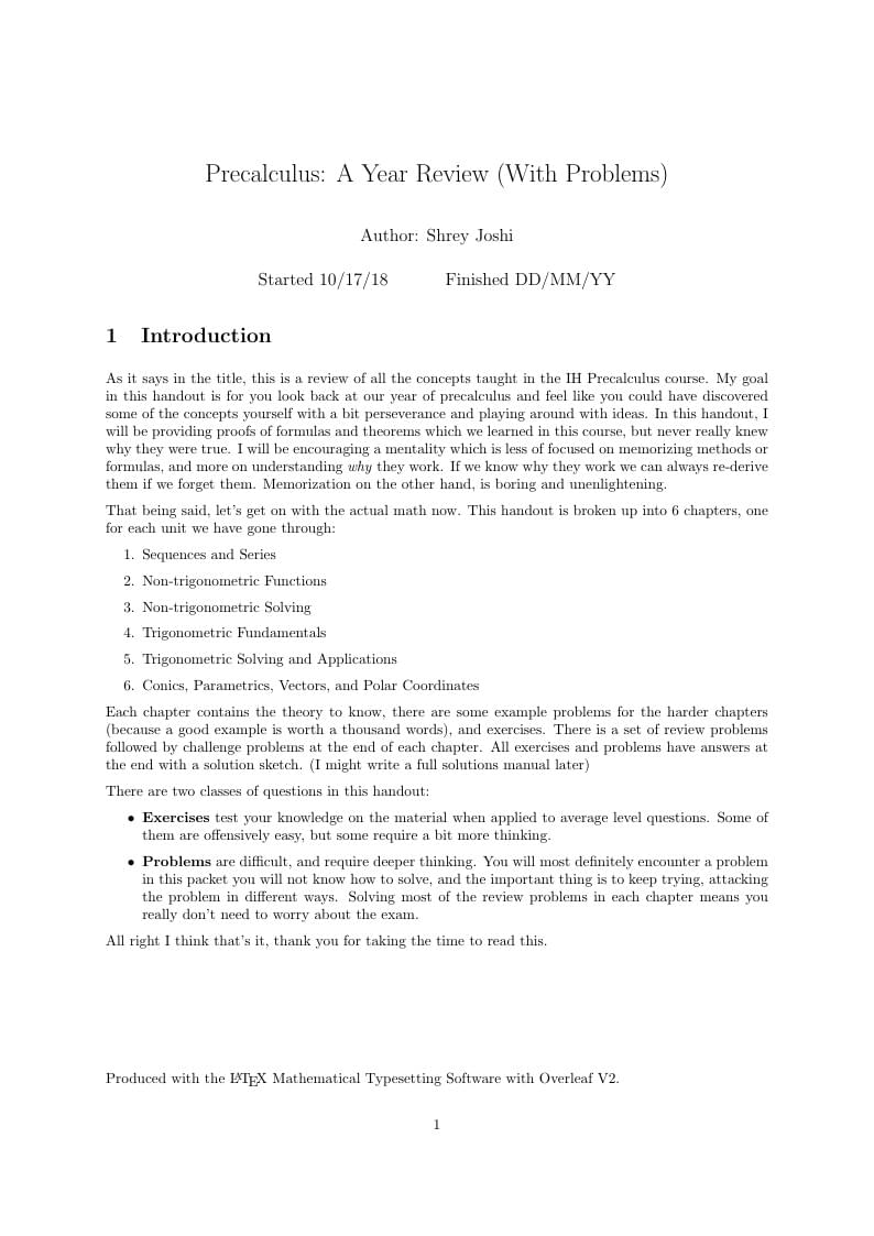
Precalculus: A Year Review (With Problems)
Author:
Shrey Joshi
Last Updated:
7년 전
License:
Creative Commons CC BY 4.0
Abstract:
Unfinished review of precal

\begin
Discover why over 25 million people worldwide trust Overleaf with their work.
Unfinished review of precal

\begin
Discover why over 25 million people worldwide trust Overleaf with their work.
\documentclass[a4paper]{article}

\usepackage{fullpage} % Package to use full page
\usepackage{parskip} % Package to tweak paragraph skipping
\usepackage{tikz} % Package for drawing
\usepackage{amsmath}
\title{Precalculus: A Year Review (With Problems)}
\author{Author: Shrey Joshi}
\date{Started 10/17/18 \quad \quad \quad Finished DD/MM/YY}

\begin{document}


\maketitle

\section{Introduction}
As it says in the title, this is a review of all the concepts taught in the IH Precalculus course. My goal in this handout is for you look back at our year of precalculus and feel like you could have discovered some of the concepts yourself with a bit perseverance and playing around with ideas. In this handout, I will be providing proofs of formulas and theorems which we learned in this course, but never really knew why they were true. I will be encouraging a mentality which is less of focused on memorizing methods or formulas, and more on understanding \textit{why} they work. If we know why they work we can always re-derive them if we forget them. Memorization on the other hand, is boring and unenlightening.

That being said, let's get on with the actual math now. This handout is broken up into 6 chapters, one for each unit we have gone through:
\begin{enumerate}
\item Sequences and Series
\item Non-trigonometric Functions
\item Non-trigonometric Solving
\item Trigonometric Fundamentals
\item Trigonometric Solving and Applications
\item Conics, Parametrics, Vectors, and Polar Coordinates
\end{enumerate}
Each chapter contains the theory to know, there are some example problems for the harder chapters (because a good example is worth a thousand words), and exercises. There is a set of review problems followed by challenge problems at the end of each chapter. All exercises and problems have answers at the end with a solution sketch. (I might write a full solutions manual later)

There are two classes of questions in this handout:
\begin{itemize}
    \item \textbf{Exercises} test your knowledge on the material when applied to average level questions. Some of them are offensively easy, but some require a bit more thinking.
    \item \textbf{Problems} are difficult, and require deeper thinking. You will most definitely encounter a problem in this packet you will not know how to solve, and the important thing is to keep trying, attacking the problem in different ways. Solving most of the review problems in each chapter means you really don't need to worry about the exam.
\end{itemize}

All right I think that's it, thank you for taking the time to read this.

\vfill
\text{Produced with the \LaTeX \ Mathematical Typesetting Software with Overleaf V2.}

\newpage
\section{Sequences and Series}
\subsection{Sequences}

\textbf{Definition 1)} A \textbf{Sequence} is a numbered collection of numbers which follow a certain pattern. For example:
$$p_n = 2, 3, 5, 7, 11, 13, 17, 19, 23, 29, 31, ... $$
These are the primes. We can denote the $n$th term of this sequence with the notation $p_n$. (i.e.
$p_3=5$, $p_7=17$, etc.).

\textbf{Definition 2)} An \textbf{Arithmetic Sequence} is defined by a starting number and a common difference. The common difference is added to a particular term in a sequence to obtain the next term. A general arithmetic sequence with a first term $a$ and a common difference $d$ has the form
$$a_n = a, a+d, a+2d, a+3d, a+4d, a+5d, ...$$
We can derive a formula for the $n$th term in arithmetic sequence. Note that in the $n$th term we add $d$, the common difference $n-1$ times to $a$, we can say
$$a_n=a+(n-1)d$$

\textbf{Definition 3)} A \textbf{Geometric Sequence} is defined by a starting number and a common ratio.
The common ratio is  multiplied by a particular term in the sequence to obtain the next term. A general
geometric sequence with a starting number $a$ and common ratio $r$ has the form
$$a_n=a, ar, ar^2, ar^3, ar^4, ar^5, ...$$
Just like arithmetic sequences, we can find a general formula for the $n$th term of a geometric sequence.
Since we are multiplying the $r$, the common ratio, $n-1$ times to $a$ for the $n$th term, we can say
$$a_n=a_1r^{n-1}$$

\textbf{Definition 4)} A \textbf{Recursive Formula} is one that defines each term in terms of a preceding term or terms. For example:
$$f(1)=1 \qquad \text{and} \qquad f(n+1)=f(n)+2$$
This is a recursive formula for the sequence $1, 3, 5, 7, 9, \cdots$. To find the next term in a sequence with a recursive formula you must find the term before it.

\textbf{Definition 5)} An \textbf{Explicit Formula} is a formula that defines the $n$th term in terms of $n$. Unlike recursive formulas we can find the $1000$th term just by plugging in $1000$ into some expression. We don't need to find any other term. We can convert recursive formulas to explicit formulas to make it easier to find a certain term in the sequence. An example of an explicit formula is the one that decirbes the sequence mentioned above.
$$f(n)=2n-1$$

\textbf{Example 1)} \\
Define an arithmetic sequence $a_n$ with 5th term $13$ and 17th term $37$. Find the value of \\
a) The first term, $a_1$ \\
b) The common difference, $d$ \\
c) The $42$nd term

<Write Solution>

\textbf{Example 2)} \\
Define a geometric sequence $a_n$ with 3rd term $45$ and 7th term $3645$. Find the value of \\
a) The first term, $a_1$ \\
b) The common ratio, $r$ \\
c) The $5$th term

<Write Solution>

\textbf{Exercise 1)} \\
<Easy thing here>

\textbf{Exercise 2)} \\
Another thing thats easy.

\textbf{Exercise 3)} \\
Find a formula for the arithmetic sequence $1+2+3+\cdots+n$.

\textbf{Exercise 4)} \\
The $2018$th term of a geometric sequence is $25$ and the $2020$th term is $36$. Find the $2019$th term (It's possible to do this without finding the common ratio or the first term).

\textbf{Exercise 5)} \\
The common difference of an arithmetic sequence, $a_n$ is equal to the common ratio of a geometric sequence, $b_n$. Given that the first term of both sequences is equal to $7$ and $\frac{b_2}{a_2}=14$, find $b_2-a_2$.

\subsection{Series}

\textbf{Definition 6)}  An \textbf{Arithmetic Series} is just the sum of the terms in an arithmetic sequence. To find the sum, we take the average of the first and last term, and multiply by the number of terms there are.

$$\underbrace{(a)+(a+d)+(a+2d)+\cdots+(a+(n-1)d)}_{\text{There are }n \text{ terms here}}=n\left(\frac{a+a+(n-1)d}{2}\right)=\boxed{n\left(\frac{2a+(n-1)d}{2}\right)}$$

\textbf{Definition 7)} A \textbf{Geometric Series} is the sum of the terms in a geometric sequence
To find this sum, we do something clever. Let's start by saying our sequence has a sum of $S$.

$$S=a+ar+ar^2+\cdots+ar^{n-1}$$
Multiplying by $r$ we get
$$Sr=ar+ar^2+ar^3+\cdots+ar^{n}$$
Subtracting $S$ from $Sr$ gives
$$Sr-S=(ar+ar^2+ar^3+\cdots+ar^{n})-(a+ar+ar^2+\cdots+ar^{n-1})$$
Note that all the terms cancel except for $a$ and $ar^{n}$.
$$Sr-S=ar^{n}-a$$
Factoring both sides we get
$$S(r-1)=a(r^n-1) \longrightarrow \boxed{S=\frac{a(r^n-1)}{r-1}}$$

You may have also seen this as $\frac{a(1-r^n)}{1-r}$. This and the expression above are one and the same.

\textbf{Definition 8)} An \textbf{Infinite Geometric Series} is just the sum of a geometric sequence that never ends. This sum only converges
if and only if $|r|<1$ where $r$ is  the common ratio (if not then each term is bigger than the last and the sum diverges). To find the formula for this
sum let's consider what happens to our finite geometric series formula as the number of terms tends to infinity. Since $|r|<1$, we know that as
$n$ tends to infinity, $r^n$ tends to $0$. Therefore we can replace $r^n$ with $0$. Hence we get
$$\lim_{n \rightarrow \infty}{\frac{a(1-r^n)}{1-r}} = \frac{a(1-0)}{1-r}=\boxed{\frac{a}{1-r}}$$

\textbf{Exercise 6)} In Definition 6 we took the limit of the sum of a finite geometric series as the number of terms tended to
infinity to find that the sum of an infinite geometric series is $\frac{a}{1-r}$. Prove this same formula differently using the method we used
to find the sum of a finite geometric series in Definition 5.
\subsection{Sigma Notation and Binomial Theorem}

\textbf{Definition 9)} \textbf{Sigma Notation} is a concise way to represent a long sum with each term of the sum only slightly different. Here's an example:

$$\sum_{i=1}^{10}=1+2+3+4+5+6+7+8+9+10=55$$

We take the dummy variable (here it is $i$), set it to equal to the starting value and sum every expression inside the sigma until our dummy variable reaches the upper limit. In this case, the starting value is $1$, then ending value is $10$ and the expression is $k$. In general we have

$$\sum_{i=a}^{b}{f(i)}=f(a)+f(a+1)+f(a+2)+\cdots+f(b-1)+f(b)$$

where $b>a$ (In our first example we had $a=1$, $b=10$, and $f(i)=i$ but we can have $a$ and $b$ holding any integer value and $f(i)$ being any function).

There are some properties of the sigma you should be familiar with. The first is that if two sigmas have the same lower and upper bounds then you can merge them into one sigma by adding the expressions. Here's an example:

$$\sum_{k=1}^{101}{k+7}+\sum_{k=1}^{101}{k^2-4} = \sum_{k=1}^{101}{k+7+k^2-4}=\sum_{k=1}^{101}{k^2+k+3}$$

Of course, you can also split sigmas this way.

$$\sum_{k=1}^{55}{k^2+k+1}=\sum_{k=1}^{55}{k^2} + \sum_{k=1}^{55}{k} + \sum_{k=1}^{55}{1}$$

In Exercise 5 you found a formula for $1+2+3+\cdots+n$. This was $n(n+1)/2$. We can find a similar formula for $1^2+2^2+3^3+\cdots+n^2$, and in general we can find a formula for $1^k+2^k+3^k+\cdots+n^k$ for any integer $k$. It pains me to do so but I will just list the formulas here without proof because I don't want to make this section overly long. If you're curious about why these formulas are true then search it up.

$$1^2+2^2+3^2+\cdots+n^2=\frac{n(n+1)(2n+1)}{6} \qquad \qquad \text{and} \qquad \qquad 1^3+2^3+3^3+\cdots+n^3=\left(\frac{n(n+1)}{2}\right)^2$$

\textbf{Definition 10)} The \textbf{Binomial Theorem} is a neat method to expand a binomial $(a+b)^n$. I would like to build this theorem up from scratch because if I display it then prove it, the proof will seem a bit contrived.

Note that

$$(a+b)^n=\underbrace{(a+b)(a+b)(a+b)\cdots(a+b)}_{\text{There are }n\text{ instances of }(a+b)}$$

Repeatedly using the distributive property, we see that for a term $a^{k}b^{n-k}$, we must choose $k$ of the $n$ terms to contribute an $a$ to the term, and then each of the other $n-k$ terms of the product must contribute a $b$. Thus, the coefficient of $a^{k}b^{n-k}$ is the number of ways to choose $k$ objects from a set of size $n$. It turns out there is function for this called the \textit{choose} function. The number of ways to choose $k$ objects from $n$ objects is

$$_{n} C_{k} = \binom{n}{k} = \frac{n!}{k!(n-k)!}$$


Here, $_{n} C_{k}$ and $\binom{n}{k}$ are just two different notations which describe the same thing. I will be using $\binom{n}{k}$, however, because it looks cooler.

Now that we know the coefficient, we can construct the entire term to be $\binom{n}{k}a^{k}b^{n-k}$. We can write

$$(a+b)^n=\binom{n}{1}a^{1}b^{n-1} + \binom{n}{2}a^{2}b^{n-2} + \binom{n}{3}a^{3}b^{n-3} + \cdots + \binom{n}{n}a^{n}b^{1}$$

This is the statement of the binomial theorem.

\textbf{Exercise 7)} Write the binomial theorem in sigma notation.

\textbf{Exercise 8)} Find the coefficient of $x^3y^3$ in the expansion of $(x+y)^6$.
\subsection{Review Problems}

\subsection{Challenge Problems}

\newpage

\section{Non-Trigonometric Functions}

\subsection{Function Properties}

Since the curriculum for this unit is pretty boring, you will find that this handout is quite short. The following is just a review of stuff in ALG 2.

\textbf{Definition 1)} A \textbf{Function} is something the maps an input value to exactly one output value. We say a function is \textbf{bijective} if every possible output can reached by exactly one input. You may have also heard of this as a one-to-one correspondence. The simplest example of a bijective function is $f(x)=x$. Here, every output can be reached by exactly one input, namely, itself. $f(x)=x^2$ is NOT a bijective function because both $f(\sqrt{x})$ and $f(-\sqrt{x})$ are equal to $x$. A function is bijective if and only if it passes both the "vertical line test" and the "horizontal line test".

\textbf{Definition 2)} A \textbf{Domain} of a function is a set of numbers for which the function is defined. The domain of $f(x)=x$ is all real numbers. However, the domain of $f(x)=\sqrt{x}$ is not all real numbers because we cannot have the square of root of a negative number. We say the function is not defined if $x$ is negative so the domain is all non-negative numbers. Finding the domain is fairly easy, we try to find inputs such that we break some rule in math (the two main ones are dividing by $0$ and square rooting a negative number).

\textbf{Definition 3)} The \textbf{Range} of a function is the set of all numbers which can be outputted from the function. The range of $f(x)=x$ is all real numbers. The domain of $|x|$, however, is only the non-negative numbers since an absolute value can never be less than $0$. Range can be a bit harder to find than domain.

\textbf{Definition 4)} An \textbf{Intercept} of a function is where it crosses an axis, whether that be the $x$ or $y$ axis. These are easy to find. For the $y$ intercept we just plug in $0$ into the function. For the $y$ intercept we find an input for which the output is $0$. (Make sure you see why). Some functions may have just an $x$ intercept, just a $y$ intercept, or neither.

\textbf{Definition 5)} The \textbf{Asymptote} of a function is the imaginary line that a function gets closer to as either $x$ or $y$ tend to infinity. There are two types of these, horizontal, and vertical.

\textbf{Horizontal Asymptotes} are lines that the function approaches as $x$ tends to $\infty$ or $-\infty$. They always take the form of $y=k$ for some constant $k$. Horizontal asymptotes are basically end behavior of the function. If $f(x)$ tends to a real value as $x$ tends to $\infty$ or $-\infty$ then the horizonatal asymptote is $y=k$. If not, then we don't have a horizontal asymptote. An example of a function with a horizontal asymptote is $f(x)=1/x$. The asympotote is $y=0$ since as $x \rightarrow \infty$ ($x$ tends to $4\infty$), $y \rightarrow 0$.

\textbf{Vertical Asymptotes} are vertical lines the function approaches as $x$ tends to some value which is not $\infty$ or $-\infty$. An example is $y=\frac{1}{(x-3)}$. The vertical asympotote is $x=3$ because as $x$ gets closer and closer to $3$ the function resembles this line more and more.

\textbf{Definition 6)} The \textbf{Extrema} of a function are the points at which the function stops increasing and starts decreasing or vice versa. We can find extrema of a function by differentiating it, setting the resulting expression equal to $0$ and solving for $x$, but since this is not a calculus review just use your calculator's maximum/minimum feature for it.

\textbf{Definition 7)} The \textbf{Holes} of a function are points at which the function is undefined. For example, in the graph of $\frac{1}{x-6}$, the point $x=6$ is a hole because $\frac{1}{0}$ is not defined. Another example is the point $x=4$ in the graph of $f(x)=\frac{2x(x-4)}{x-4}$ or the point $x=0$ in the graph $f(x)=x^x$.

Don't try and memorize all the stuff on this page. Rather, if you need to, try to find spatial connections of these attributes, identify them on graphs of some functions.

\textbf{Exercise 9)} Find each of the following attributes...
\begin{itemize}
    \item Domain
    \item Range
    \item Asymptotes
\end{itemize}
...for each of the following functions
\begin{itemize}
    \item $f(x)=x^3$
    \item $f(x)=x^{-1}$
    \item $f(x)=\sqrt{x}$
    \item $f(x)=b^x$ for $b>1$
    \item $f(x)=\log_{b}{x}$ for $b>1$
\end{itemize}

\subsection{Function Transformations And Other Stuff Like It}

Lol no this is boring (and you should have an idea of it from ALG 2)

\subsection{More Interesting Stuff In This Unit That I Can Write About Without Pulling My Hair In Frustration}

This consists of the following:
\begin{itemize}
    \item Rational Root Theorem (RRT)
    \item Synthetic Division
\end{itemize}
\end{document}