Hw4
Author:
Arpit Gupta
Last Updated:
12년 전
License:
Creative Commons CC BY 4.0
Abstract:
AML

\begin
Discover why over 25 million people worldwide trust Overleaf with their work.

\begin
Discover why over 25 million people worldwide trust Overleaf with their work.
\documentclass[12pt]{amsart}

\pagestyle{empty}
\textwidth 7.5in
\textheight 9in
\oddsidemargin -0.3in
\evensidemargin -0.2in
\topmargin -0.2in

\newcommand{\norm}[1]{\Vert #1 \Vert}
\newcommand{\Rn}{\R^n}
\newcommand{\Rm}{\R^m}
\newcommand{\R}{{\mathbb{R}}}
\newcommand{\grad}{\nabla}
\newcommand{\Rnn}{\R^{n\times n}}
\newcommand{\map}[3]{#1:#2\rightarrow #3}
\newcommand{\half}{\frac{1}{2}}
\newcommand{\Rmn}{\R^{m\times n}}
\newcommand{\tpose}[1]{#1^{\scriptscriptstyle T}}
\newcommand{\indicator}[2]{\delta\left(#1 \mid #2 \right)}


\usepackage{color}
\newcommand{\blue}[1]{\textcolor{blue}{#1}}
\newcommand{\red}[1]{\textcolor{red}{#1}}


\newcommand{\prox}{\mathrm{prox}}
\newcommand{\logit}{\mathrm{logit}}


\usepackage{amsmath,epsfig,amssymb}
%\input{macros}
%\input{macros2}

\begin{document}
{\Large Name: Arpit Gupta AG3418}  \\
\begin{center}
\Large COMS 4772 \hskip 2in Homework Set 4
\end{center}
\bigskip


\noindent

\begin{enumerate}

\item You may use the fact that {\it expectation is a linear operator}.
\begin{enumerate}
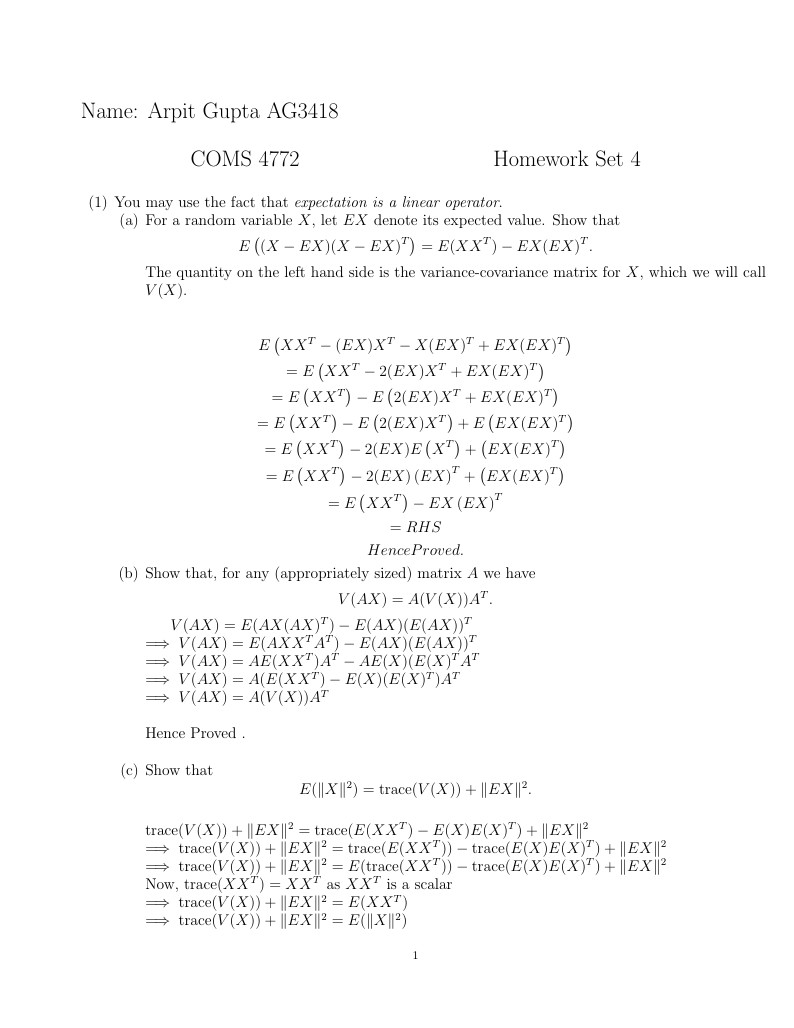
\item For a random variable $X$, let $EX$ denote its expected value. Show that
\[
E\left((X-EX)(X-EX)^T\right) = E(XX^T) - EX(EX)^T.
\]

The quantity on the left hand side is the variance-covariance matrix for $X$, which we will call $V(X)$.\\ \\
\[
E\left(XX^T - (EX)X^T - X (EX)^T + EX(EX)^T \right)
\]
\[
=E\left(XX^T -2 (EX)X^T + EX(EX)^T \right)
\]
\[
=E\left(XX^T\right) - E \left( 2 (EX)X^T + EX(EX)^T \right)
\]
\[
=E\left(XX^T\right) - E \left( 2 (EX)X^T \right) + E \left( EX(EX)^T \right)
\]
\[
=E\left(XX^T\right) - 2 (EX) E \left(X^T \right) + \left( EX(EX)^T \right)
\]
\[
=E\left(XX^T\right) - 2 (EX) \left(EX\right)^T  + \left( EX(EX)^T \right)
\]
\[
=E\left(XX^T\right) - EX\left(EX\right)^T
\]
\[
=RHS
\]
\[
Hence Proved .
\]

\item Show that, for any (appropriately sized) matrix $A$ we have
\[
V(AX) = A(V(X))A^T.
\]
$ \ \ \ \ \ V(AX) = E(AX(AX)^T) - E(AX)(E(AX))^T$ \\
$\implies V(AX) = E(AXX^TA^T) -E(AX)(E(AX))^T $ \\
$\implies V(AX) = AE(XX^T)A^T -AE(X)(E(X)^TA^T $ \\
$\implies V(AX) = A (E(XX^T) - E(X)(E(X)^T)A^T $ \\
$\implies V(AX) = A (V(X))A^T $ \\

Hence Proved . \\

\item Show that
\[
E(\|X\|^2) = \mbox{trace}(V(X))  + \|EX\|^2.
\]
\null \\
$ \ \ \ \ \  \mbox{trace}(V(X))  + \|EX\|^2  = \mbox{trace}(E(XX^T) -E(X)E(X)^T) + \|EX\|^2 $ \\
$\implies \mbox{trace}(V(X))  + \|EX\|^2  = \mbox{trace}(E(XX^T)) - \mbox{trace}(E(X)E(X)^T) + \|EX\|^2 $ \\
$\implies \mbox{trace}(V(X))  + \|EX\|^2  = E(\mbox{trace}(XX^T)) - \mbox{trace}(E(X)E(X)^T) + \|EX\|^2 $ \\
Now, $\mbox{trace}(XX^T) = XX^T$ as $XX^T$ is a scalar \\
$\implies \mbox{trace}(V(X))  + \|EX\|^2  = E(XX^T) $ \\
$\implies \mbox{trace}(V(X))  + \|EX\|^2  = E(\|X\|^2) $ \\

\item Solve the stochastic optimization problem
\[
\min_y E\|X - y\|_2^2,
\]

where $X$ is a random vector, and the expectation is taken with respect to $X$.
What is the minimizer? What's the minimum value? \\\\

Answer : \\
\[
\min_y ( E\|X - y\|_2^2
\]
\[
= \min_y ( E((X - y)(X-y))^T )
\]
\[
= \min_y ( E(XX^T - 2Xy^T + yy^T )
\]
\[
= \min_y ( E(XX^T) -2y^TE(X) + yy^T )
\]

Take gradeient of above equation and equate to zero.
\[
\grad ( E(XX^T) -2y^TE(X) + yy^T ) = 0
\]
\[
\implies -2E(X) + 2y = 0
\]
\[
\implies y = E(X)
\]

\end{enumerate}

\item Frobenius norm estimation. Suppose we want to estimate
\[
\|A\|_F^2 = \mbox{trace}(A^TA)
\]
of a large matrix $A$. One way to do this is to hit $A$ by random vectors $w$, and then measure
the resulting norm.
\begin{enumerate}
\item Find a sufficient conditions on a random vector $w$  that ensures
\[
E \|Aw\|^2 = \|A\|_F^2.
\]
Prove that your condition works. \\
Answer : \\
\[
\|A\|_F^2 = \mbox{trace}(A^TA)
\]
\[
\implies \|A\|_F^2 = \mbox{trace}((A^TIA))
\]
\[
\implies \|A\|_F^2 = \mbox{trace}(A^TE(w^Tw)A)
\]
where w, is a random variable with E(W) = 0 , and Var(w) = 1 \\
\[
\implies \|A\|_F^2 = \mbox{trace}(A^TE(w^Tw)A)
\]
\[
\implies \|A\|_F^2 = \mbox{trace}(E \left( (wA)^TwA \right) )
\]
As trace is a linear operator, \\
\[
\implies \|A\|_F^2 = E \left( \mbox{trace}((wA)^TwA ) \right)
\]
\[
\implies \|A\|_F^2 = E \left( \mbox{trace}(\|Aw\|^2 ) \right)
\]
Now, $\|Aw\|$ will, be a $1X1$ scalar , therefore it is same as its trace. \\
\[
\implies \|A\|_F^2 = E \|Aw\|^2
\]

Hence Proved. \\
And w, mjst be  a random variable with E(W) = 0 , and Var(w) = 1 \\


\item What's a simple example of a distribution that satisfies the condition you derived above? \\

White Gaussian Noise is an example of $w$ that will satisy above condition. \\

\item Explain how you can put the relationship you found to practical use to estimate $\|A\|_F^2$ for a large $A$.
In particular, you must explain how to estimate $\|A\|_F^2$ more or less accurately, depending on the need. \\

Answer : \\ \\

We can take Expected value of $\|Aw\|^2 $ by choosing different $w$ multiple times, and averaging over the values of  $\|Aw\|^2 $ By increasing the number of times we sample $w$, we can achieve higer accuracy, as the sampling count approaches infinity, we will exactly match $\|A\|_F^2$  \\

\item Test out the idea in Matlab. Generate a random matrix $A$, maybe 500 x 1000. Compute its frobenius norm
using \verb{norm(A, 'fro'){ command.  Compare this to the result of your approach. Are they close? Is your approach faster? \\

Answer : \\

It is faster when number of times $w$ is less than  . As the number of times I sample $w$ is increased, accuracy increases. \\

\end{enumerate}


\item Consider again the logistic regression problem.
Included with this homework is the covtype dataset (500K examples, 54 features).

Consider again the logistic regression formulation:
\[
\min_\theta \frac{1}{N}\sum_{i=1}^N \log(1+\exp(\tilde x_i^T \theta)) + \lambda\|\theta\|_2
\]
where $\tilde x_i = -y_i x_i$ and you can take $\lambda = 0.01$ (small regularization).

Implement a stochastic gradient method for this problem.

Use the following options for step length:
\begin{enumerate}
\item Pre-specified constant
\item Decreasing with the rule $\alpha(k) \propto \frac{1}{k}$ (with some initialization)
\item Decreasing with rule $\alpha(k) \propto \frac{1}{k^{0.6}}$ (with some initialization) \\
\end{enumerate}

Divide covtype into two datasets, 90\% training and 10\% testing. Tune each of the three previous step size routines
(i.e. adjust the constant or the constant initialization) until you are happy each one performs reasonably well.
Make a graph showing the value of the {\it test likelihood} as a function of the iterates for each of the three strategies. \\


\item (BONUS)

\begin{enumerate}
\item Change the counting in the previous problem to be as a function of {\it effective passes through the data},
rather than iterations. For example, five iterations with batch size 1 should be no different than one iteration with batch size 5 in this metric. \\

\item For the pre-specified constant step length strategy, compare test likelihood as a function of effective passes through the data
for different random batch sizes, e.g. 1, 10, and 100. \\

\item Again for pre-specified constant step length strategy, implement a growing batch size strategy, where the size of the batch
increases with iterations. Can this strategy beat the fixed batch size strategy, with respect to effective passes through the data? \\


\end{enumerate}

\end{enumerate}
\end{document}